
Hence, Top 50 Excel formulas is essential to learn for anyone who works with numbers in their office or business. Scope of Excel is tremendous, whether we are an aspiring analyst, a business professional, or simply use Excel for our personal finance and work.
Excel is a powerful tool that can help us make better decisions and save us hours of work. It’s not just about grids and charts. We’ll dissect the Top 50 Excel formulas that every analyst and corporate employee needs to be aware of in this post. Even if we are just starting out, we will feel comfortable using these formulas because we have provided brief explanations and easy-to-understand examples for every formula. Let’s get started and turn Excel into our new superpower!
1. SUM()
Description:
This formula is used to add numbers or the values in a range. The range can be a row or a column.
Example:=SUM(10, 20, 30)
Explanation:
Adds 10 + 20 + 30. Hence the result is 60.
Similarly, =SUM(A1:A3) will add all the numbers from cells A1 to cell A3.
2. AVERAGE()
Description:
Average is used to find the average (mean) of given numbers.
Example:=AVERAGE(10, 20, 30)
Explanation:
(10 + 20 + 30) ÷ 3 = 60 ÷ 3 = 20.
It will first calculate the sum of these numbers and then divide it by the number (count) of values.
3. MIN()
Description:
It will return the smallest number in a set of numbers.
Example:=MIN(5, 2, 8)
Explanation:
As we can see that among 5, 2, and 8, the smallest number is 2. Hence, MIN scanned all the numbers and picked the lowest one.
4. MAX()
Description:
Is used to return the largest number in a set of numbers.
Example:=MAX(5, 2, 8)
Explanation:
Clearly, among 5, 2, and 8, the highest number is 8.
5. COUNT()
Description:
COUNT is used to count how many numbers are there in a list.
Example:=COUNT(10, "Hello", 20, "")
Explanation:
Since only 10 and 20 are numbers, so COUNT will ignore text, which is ‘Hello’ in this case and blanks.
Result = 2.
6. COUNTA()
Description:
This version of count tells us how many non-empty values are there in the set.
Example:=COUNTA(10, "Hello", "")
Explanation:
As we can see, 10 and “Hello” are non-empty. The blank (“”) gets ignored.
Result = 2.
7. COUNTBLANK()
Description:
It counts the number of empty cells in a range.
Example:
If A1:A3 = [10, “”, “Hello], then=COUNTBLANK(A1:A3)
Explanation:
Certainly, only one cell (the 2nd one) is empty.
Result = 1.
8. IF()
Description:
If will return one value if a condition is TRUE, another if FALSE. It is a very useful formula. To understand the syntax, let’s look at below example where we are trying to write ‘Yes’ if 10>5 and ‘No’ if the it is not. Practice this well as it one of the most important Top 50 Excel Formulas.
Example:=IF(10>5, "Yes", "No")
Syntax is – IF(logical test, ‘result if true’, ‘result if false’)
Explanation:
10 is greater than 5, so the condition is TRUE.
It returns “Yes”.
9. IFS()
Description:
This is the next step of IF. With IFs we can check multiple conditions at once. In below example, we will test multiple conditions. If 90>100, result should be ‘A’ and the formula will stop there. if not, it will proceed to next test which is 90>80 and result should be ‘B’ and formula stops. This will continue as long as we keep giving logical tests.
Example:=IFS(90>100, "A", 90>80, "B", 90>70, "C")
Explanation:
-
90 > 100 → FALSE
-
90 > 80 → TRUE → hence it returns “B” and will not be checking further.
10. AND()
Description:
AND returns TRUE if all conditions are TRUE. In below example, we will give 2 conditions and see what happens.
Example:=AND(10>5, 8<12)
Explanation:
Since both the conditions we gave are TRUE (10>5 and 8<12), so AND returns TRUE. We can give more than 2 conditions too.
11. OR()
Description:
OR is used to return TRUE if at least one condition is TRUE. Think of it as opposite of AND.
Example:=OR(10<5, 8<12)
Explanation:
-
10<5 → FALSE
-
8<12 → TRUE
Here one condition is TRUE, so OR returns TRUE. Try to compare it with AND for your understanding.
12. NOT()
Description:
It is not a very popular formula but useful to know as it helps in some cases. We can use it for reversing the result: TRUE becomes FALSE and vice versa.
Example:=NOT(10>5)
Explanation:
Even tough 10>5 is TRUE, but NOT will flip it to FALSE.
13. ISBLANK()
Description:
It is used to check if a cell is empty.
Example:=ISBLANK(A1)
Explanation:
If there is no value in A1, it will return TRUE else it will return FALSE.
14. ISNUMBER()
Description:
It checks if a cell contains a number.
Example:=ISNUMBER(A1)
Explanation:
it will return TRUE If A1 contains a number like 10 or 5.5, else it will show FALSE.
15. ISTEXT()
Description:
Checks if there is text in a cell.
Example:=ISTEXT("Hello")
Explanation:
Since “Hello” is text, it returns TRUE. It will return FALSE for numbers and special characters like &, *, #.
16. VLOOKUP()
Description:
VLOOKUP is the most important Top 50 Excel formulas. It searches for a value in the first column and returns a value in the same row. Let’s see the first table. We have fruits and their prices. Now if someone asks us the price of Apple or Mango we can easily check the table and tell. However, when the list of fruits is very long, say 10,000 fruits and someone asks us to check the prices of 3500 fruits from the list, we will not be able to do it manually.
Hence we need VLOOKUP.
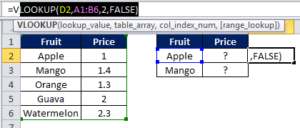
Example:=VLOOKUP(D2, A1:B6, 2, FALSE)
Explanation:
First 5 columns are A,B,C,D and E. Syntax is visible in the image. First we enter the lookup_value which is Apple in the second table (D2). This is the cell whose value we are looking for from the 1st table. Then we select the range where the original table is located (A1:B6). Then we enter the column no. of original table where the value is located. In this case, this is the 2nd column of 1st table where price is located. Finally we write FALSE if we want exact match and TRUE for broad match. Exact match will search for Apple only and broad match will also look for spelling errors and typos.
17. SUMIF
Description:
SUMIF gives the SUM of a range based on a condition.
Example:=SUMIF(A1:A7,"Apple",B1:B7)
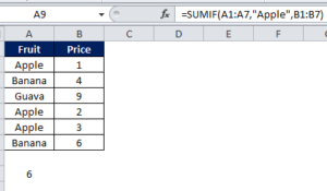
Explanation:
Syntax if =SUMIF(Range, Criteria, Sum range). Here we wanted to calculate the total cost for Apples.So we first gave the range where fruits are mentioned, then gave “Apple” as a criteria to filter this range. Finally, we gave sum range where values are located (B1:B7). Result is 6.
18. COUNTIF
Description:
Similar to SUMIF, COUNTIF will count the number of instances a fruit appears in the table.
Example:=COUNTIF(A1:A7,"Apple")
Explanation:
We get 3 as our answer. First we gave range and then the criteria.
19. INDEX()
Description:
Index basically returns the value from a given position in a range.
Example:=INDEX(A2:C5, 2, 3)
Explanation:
It will fetch the value at 2nd row and 3rd column in the range A2:C5.
20. MATCH()
Description:
It is used with Index function. It finds the position of a value in a range.
Example:=MATCH(20, A1:A5, 0)
Explanation:
Obviously if 20 is the third item in range A1:A5, MATCH will return 3.
21. CONCAT()
Description:
It is basically used for joining two or more cells together.
Example:=CONCAT("Hello ", "World")
Explanation:
Here it combines the two words into “Hello World”.
22. TEXTJOIN()
Description:
It basically joins multiple cells with a separator like comma or space.
Example:=TEXTJOIN(", ", TRUE, A1:A3)
Explanation:
It will join A1, A2, and A3 with a comma and space (“, “) between them.
23. LEFT()
Description:
Extracts specific number of characters from the left side of a text.
Example:=LEFT("Excel", 2)
Explanation:
Hence, it will take the first 2 letters: “Ex”.
24. RIGHT()
Description:
Similarly, RIGHT extracts characters from the right side of a text.
Example:=RIGHT("Excel", 2)
Explanation:
Takes the last 2 letters: “el”.
25. MID()
Description:
It extracts text from the middle of a string.
Example:=MID("Excel", 2, 3)
Explanation:
It starts characters from the 2nd letter (“x”) and thereafter it will take 3 letters → “xce”.
26. LEN()
Description:
It counts the number of characters in a string.
Example:=LEN("Excel")
Explanation:
“Excel” has 5 characters, so evidently the answer is 5.
27. TRIM()
Description:
TRIM can remove extra spaces from text, but it does not remove single spaces between words, making it very useful for cleaning data.
Example:=TRIM(" Hello World ")
Explanation:
Thus it will return “Hello World” with clean spacing.
28. UPPER()
Description:
It can convert text to uppercase.
Example:=UPPER("excel")
Explanation:
Thus it converts “excel” to “EXCEL”.
29. LOWER()
Description:
This formula can convert text to lowercase.
Example:=LOWER("EXCEL")
Explanation:
Hence it will change “EXCEL” to “excel”.
30. PROPER()
Description:
This is used to capitalize the first letter of each word.
Example:=PROPER("hello world")
Explanation:
Hence it will convert “hello world” to “Hello World”. Evidently a very useful formula for data cleaning.
31. NOW()
Description:
It can return current date and time.
Example:=NOW()
Explanation:
If today is April 9, 2025, 5 PM, it will return 09-04-2025 17:00.
32. TODAY()
Description:
This formula returns the current date but not the time.
Example:=TODAY()
Explanation:
If it is April 9, 2025 today, it will return 09-04-2025.
33. DAY()
Description:
Can extract day from a date.
Example:=DAY("09-04-2025")
Explanation:
Hence we get 9 (day part) from the date.
34. MONTH()
Description:
Similarly, MONTH returns the month of a date.
Example:=MONTH("09-04-2025")
Explanation:
Thus we get 4 (April) from the date.
35. YEAR()
Description:
It can return the year of a date.
Example:=YEAR("09-04-2025")
Explanation:
Evidently, we get 2025 from the date.
36. WEEKDAY()
Description:
It returns the day of the week in the form of a number (1 = Sunday, 2 = Monday…).
Example:=WEEKDAY("09-04-2025")
Explanation:
Evidently if April 9, 2025, is Wednesday, it will return 4.
37. DATEDIF()
Description:
This is a very useful formula. It can calculate the difference between two dates.
Example:=DATEDIF("01-01-2025", "09-04-2025", "d")
Explanation:
Thus it will auto calculate the number of days between January 1 and April 9 (98 days).
38. NETWORKDAYS()
Description:
This formula calculates the number of working days between two dates.
Example:=NETWORKDAYS("01-04-2025", "09-04-2025")
Explanation:
Hence it counts weekdays and excludes weekends (and optionally holidays).
39. TEXT()
Description:
Converts numbers and dates as text.
Example:=TEXT(TODAY(), "DD-MM-YYYY")
Explanation:
Thus it formats the date like “09-04-2025”.
40. ROUND()
Description:
It can round off a number to a specified number of digits.
Example:=ROUND(5.6789, 2)
Explanation:
Evidently it will round off 5.6789 to 5.68.
41. ROUNDUP()
Description:
It can round a number up.
Example:=ROUNDUP(5.123, 2)
Explanation:
Hence it rounds up 5.123 to 5.13.
42. ROUNDDOWN()
Description:
It is the opposite of ROUNDUP. It rounds a number down.
Example:=ROUNDDOWN(5.987, 2)
Explanation:
So it rounds down 5.987 to 5.98.
43. CEILING()
Description:
CEILING function rounds a number up to the nearest given multiple.
Example:=CEILING(5.2, 1)
Explanation:
Thus it will round 5.2 up to the nearest multiple of 1 → 6.
44. FLOOR()
Description:
Rounds a number down to the nearest multiple.
Example:=FLOOR(5.8, 1)
Explanation:
So it rounds 5.8 down to the nearest multiple of 1 → 5.
45. MOD()
Description:
MOD can return the remainder after division.
Example:=MOD(10, 3)
Explanation:
In 10 ÷ 3 = 3, remainder 1, thus it returns 1.
46. ABS()
Description:
This formula gives the absolute value of a number (ignores negative sign).
Example:=ABS(-10)
Explanation:
Hence it converts -10 into 10.
47. POWER()
Description:
This formula raises a number to a power.
Example:=POWER(3, 2)
Explanation:
hence we get 3^2 = 9.
48. SQRT()
Description:
It returns the square root of a number.
Example:=SQRT(25)
Explanation:
Evidently, square root of 25 is 5.
49. RAND()
Description:
Basically it can generates a random number between 0 and 1.
Example:=RAND()
Explanation:
Hence, it might return something like 0.7263. It is different every time you recalculate.
50. RANDBETWEEN()
Description:
Generates a random whole number between two given numbers.
Example:=RANDBETWEEN(1, 100)
Explanation:
Accordingly it will return any whole number between 1 and 100, like 57.
Conclusion:
Congratulations! 🎉 You’ve just unlocked Top 50 Excel Formulas. We now have a solid basis to analyze data more quickly and intelligently, from simple calculations like SUM and AVERAGE to more sophisticated tools like VLOOKUP, INDEX-MATCH, and IFERROR.
Keep in mind that the more we use these top 50 excel formulas, the more natural they will feel and the more adept we will be at identifying details that others might overlook. You’ll soon be able to handle even the most difficult Excel tasks like a pro if you keep this list close at hand and experiment with different formula combinations. Have fun with your analysis!
Learn more about Top 50 Excel formulas at – https://support.microsoft.com/en-us/excel
Also check out our articles on SQL –
Good
Good.
Good.
Very good.
Awesome.
Good.
Very good.
Very good.
Good.
Good.