
Power Query in Excel is a very handy tool that can save us hours of manual work while working with unorganized data or while performing repetitive steps. All the Excel versions (2016 and later) have this powerful feature built into them. Power Query in Excel let’s us clean, organize and transform data without having to write any complicated formulas or VBA macros. All we have to do is understand the steps and it gets done with a few simple clicks.
In this article, we will explore how to perform the basic steps of Power Query in Excel, then we will move to intermediate tasks and then practice with step-by-step tutorial and examples. Please download and open the file above as all the examples in this article have been discussed using the data from that Excel only.
👉 Download the Excel File – Before we start, please download the Excel sheet used in this tutorial.
📘 What is Power Query in Excel?
As discussed above, Power Query helps us to clean, organize and transform data. We can get the same task done manually as well using VLOOKUP and Pivot Tables but that will take more time. In Power Query, we can also save the steps for future use. We can find the Power Query feature in Excel under the Data tab > Get & Transform.
Below are the 3 steps used in running Power Queries –
-
First we need to Connect to a data source (Excel, CSV, web, SQL, etc.).
-
Then transform the data (clean, filter, rename, merge, etc.).
-
Finally, load the cleaned data into Excel as a new table or into Power Pivot.
Let’s understand all 3 steps in more details.
📂 Data Used in This Tutorial on Power Query in Excel
Open the Excel sheet provided above. If you see, it has the following tabs:
-
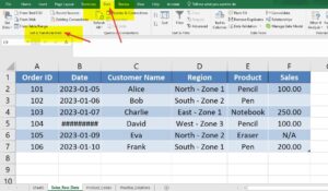
Sales_Raw_Data: This sheet has the raw data. We have these columns – order id, date, customer name, region, product, and sales amount.
-
Product_Codes: It has a table that tells us which product belongs to which category.
-
Practice_Solutions: Just a blank sheet where we can load our transformed data.
Now we will perform the 3 steps mentioned above on our dataset and load the final result back into the Excel.
🧪 Example 1: Removing Unnecessary Columns via Power Query
Goal: We will start with a very basic task to understand the Power Query in Excel interface. Task is to keep only the important columns: Date, Region, Product, and Sales in Sales_Raw_Data tab and remove / delete other columns.
Steps:
-
First select the
Sales_Raw_Datatable. -
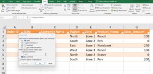
Then go to Data > Get & Transform > From Table/Range. Select the entire table. Check the ‘My table has headers column’ and click ok. We just loaded our table as a query in the editor.
-
Now in Power Query Editor, hold
Ctrland just click the columns that we want to remove (e.g.,Order ID,Customer Name). -
Then right-click > Remove Columns.
✅ Result: Thus, we cleaned our Excel by removing unnecessary columns. You may be wondering that we could have done that simply by right clicking the column and deleting it. However, this is just to understand the more complex operations of Power Queries in Excel. Let’s move to next tasks.
🧹 Example 2: Changing Column Names via Power Query in Excel
Goal: Now we will rename columns to make them more user-friendly.
Steps:
-
Double-click the column headers to rename them. Now rename as follows –
-
Change
Salesto→Sales_Amount -
Change
Productto →Product_Name
-
✅ Result: Now our column names are more standardized. As mentioned above, do not try to see the result in Excel just yet. Let’s first perform the remaining steps as below –
🔄 Example 3: Replacing Errors or Null Values via Power Query
As we can see, some rows in Sales_Amount are empty or have errors (e.g., “N/A”).
Goal: Replace nulls or errors with 0. Otherwise we will not be able to perform calculations on this data.
Steps:
-
First select the
Sales_Amountcolumn. -
Then go to Transform > Replace Values. We will see two boxes – ‘Value to find’ and ‘Replace with’.
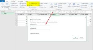 Enter “null” in the first box and
 0in the second one. Now hit ok and it will be done. You will see the new version in Power Query editor.- If you still see any error cells, just go to Home > Remove Errors or use Transform > Replace Errors.
✅ Result: We have ensured that all our sales data is now numeric and clean.
📅 Example 4: Splitting Columns via Power Query in Excel
Now let’s have a look at the Region column. it is currently in the format: "North - Zone 1". However, if we want to do zone wise analysis, like total sales in Zone 1, Zone 2 etc, we won’t be able to do it.
Goal: We should split it into Main_Region and Sub_Zone So that we can do the analysis region wise and zone wise too.
Steps:
-
First select the
Regioncolumn. -
Then go to Transform > Split Column > By Delimiter.
-
In the first drop down, choose custom and enter
" - "as the delimiter. It means Power Query in Excel will split this column into two separate columns whenever it finds.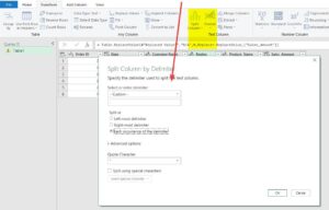
-
Rename the new columns as Region and Zone.
✅ Result: We now have two separate region fields for better analysis.
🔗 Example 5: Merging (Joining) Tables
We also have a Product_Codes table with Product_Name and Category.
Goal: Add the Category column against Product_Name column in Sales_Raw_Data tab.
Steps:
- Load Product_Codes tab to Power Query following the steps in example 1.
-
In Power Query, go to Home > Merge Queries.
-
Select
Sales_Raw_DataandProduct_Codes. -
Select
Product_Namecolumns in both the tables. -
Use a Left Join.
-
Expand the merged table to include the
Categorycolumn.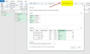
✅ Result: Hence, our dataset now includes product categories.
🧮 Example 6: Changing Data Types
Sometimes numbers get treated as text.
Goal: Ensure every cell in Sales_Amount is treated as a number.
Steps:
-
Select the
Sales_Amountcolumn. -
Go to Transform > Data Type > Decimal Number.
✅ Result: Thus, we can use this column for calculations.
📤 Loading the Transformed Data
Finally, cross check all the steps above and once our data looks good, we can proceed to loading this result back into our Excel using the steps:
-
Click Home > Close & Load To…
-
Then, choose Existing worksheet and select the
Practice_Solutionssheet. -
Click OK.
🎉 You’re done! Your clean data is certainly ready for analysis now.
🧠 Summary of Common Transformations in Power Query
| Transformation | What it does |
|---|---|
| Remove Columns | Delete unwanted data |
| Rename Columns | Make headers user-friendly |
| Replace Values | Handle missing or incorrect data |
| Split Columns | Separate text into new columns |
| Merge Queries | Join data from two tables |
| Change Data Types | Ensure correct format for analysis |
🧩 Practice Questions for Power Query in Excel
We have understood the basics of Power Query in Excel. As next steps, we can try below questions on our own using the same file:
-
Remove rows where
Sales_Amountis 0. -
Then, filter data to only show
Southregion sales. -
Then, move to Group by
Categoryand sum the totalSales_Amount. -
Now, sort the final data by
Sales_Amountin descending order. -
At last, add a column that calculates 10% commission from each
Sales_Amount.
If we get stuck anywhere, we can reload the original data anytime using Home > Refresh Preview in Power Query.
✅ Why Use Power Query in Excel?
-
No formulas required
-
Reusable steps (refresh with new data)
-
Also, it works with Excel, CSV, web, databases
-
Besides calculations, it makes reporting much faster!
📌 Final Tips
-
Power Query is non-destructive – it doesn’t change our original data.
-
Also, we can undo any step from the Applied Steps pane.
-
Additionally, we can save time by recording transformation steps once, and reapplying them anytime.
💬 Have Questions?
Alright, drop your questions in the comments! I’ll try to include more examples in a follow-up article.
If you do not have power query in your Excel, you may download from here
Also check out our other articles on –
Awesome.