")
We all are so used to of using Excel in daily work like data entry, analysis, visualization etc. However, ever since Microsoft launched Dynamic Arrays in Excel 365 and Excel 2019, Excel became much more powerful and lot more easy to use. Dynamic arrays are a set a three formulas – Filter, SORT and UNIQUE in Excel. These formulas are used individually and in combination with each other too.
They can be a game changer when it comes to boosting productivity in Excel. Lot of manual copy and pasting can be saved via these formulas. In this article, we will discuss each function in beginner level terms, learn using these for increased productivity, and also practice with real life examples.
What Are Dynamic Arrays: FILTER, SORT and UNIQUE in Excel?
Let’s start from the very basics – the meaning of dynamic array in Excel.
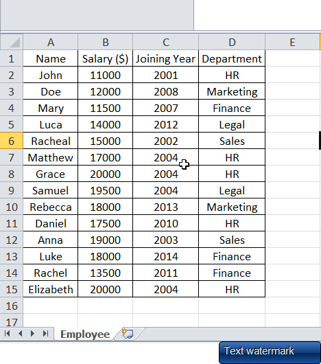
We use dynamic array formula to spill the content of selected cells into adjacent cells. For e.g., suppose we have an employee table where name, salary, joining date and department of all employees are mentioned. Now we want only the details of employees from HR department to be shown as a separate table at a new location, we can use dynamic array formulas.
Best part is the new table with only HR department employees will update automatically whenever original data changes. This saves us lot of effort on copy+paste. Now let’s dive deeper. We will use below table to discuss examples –
1. FILTER Function – Extract What You Need
Syntax:
-
array: This is the original data that we want to filter. -
include: This is the condition or rule we want to apply for filtering. -
if_empty: (Optional) It is a custom message we can show if no results are found after filtering.
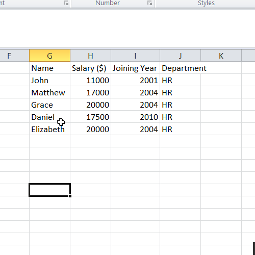
Example 1: Basic Filter
In the table shown above, we want that only the employees from HR department are shown at a new location. Type this formula at the desired location:
Result:
Example 2: Filter with Multiple Conditions
We can give multiple conditions to filter as well. For e.g., we want only the HR employees with salary >15000 to show.
Here, the * works as an AND logic.
2. SORT Function – Organize Your Data
It is used to sort a column in ascending or descending order.
Syntax:
-
sort_index: Column number that we want to sort (e.g., 2 means the second column from the left). -
sort_order: 1 would mean sort in ascending order and -1 is used to sort in descending order. -
by_col: FALSE = sort by row (optional, default and recommended), TRUE = sort by column.
Example: Sort by Salary (Descending)
This will sort the entire data by the 3rd column (Salary) in descending order.
3. UNIQUE Function – Eliminate Duplicates
We can use this formula to delete duplicate values.
Syntax:
Example 1: Unique Departments
Result:
HR
Finance
Sales
Legal
Marketing
Combine FILTER, SORT, and UNIQUE in Excel Like a Pro
We can combine these functions together for advanced applications.
Use Case: Top Unique Departments by Salary
Imagine that we are looking to achieve this:
-
Only keep people with Salaries above $10,000
-
Mention the departments of those people
-
Sort the result alphabetically
Thus, this one single formula gives you clean, sorted department names. If you find it difficult to combine these, you can write them individually too. For e.g., first write the FILTER formula, then write SORT in another cell to sort the result of UNIQUE.
Real-World Examples of FILTER, SORT and UNIQUE in Excel
Example 1: Shortlist Based on Salary
| Name | Department | Salary |
|---|---|---|
| Aditi | HR | 45000 |
| Raj | IT | 60000 |
| Meena | HR | 48000 |
| John | Sales | 50000 |
| Rahul | HR | 52000 |
| Nisha | IT | 58000 |
Objective: Display HR employees who have a salary above $47,000 in descending salary order.
Example 2: Email Campaign – Unique Customer Locations
| Name | City |
|---|---|
| Rohit | Mumbai |
| Sneha | Delhi |
| Anil | Mumbai |
| Tanya | Kolkata |
| Arjun | Delhi |
| Riya | Pune |
Find out the list of unique cities mentioned in the above table.
Additionally, we can merge it with SORT as well –
Practice Questions on FILTER, SORT and UNIQUE in Excel
Now that we have an understanding of FILTER, SORT and UNIQUE in Excel, let’s solve these practice questions on a spreadsheet –
Q1. We have a list of products with their respective prices. We want to filter those products which have a price above ₹1000.
| Product | Price |
|---|---|
| Pen | 100 |
| Chair | 1500 |
| Desk | 2500 |
| Mug | 300 |
Q2. Further, have a look at the below table. It has employee names and their respective departments. Extract the list of unique departments and sort the result alphabetically.
| Name | Department |
|---|---|
| Aditi | HR |
| Raj | IT |
| Meena | HR |
| John | Sales |
| Rahul | IT |
Q3. From this table below, extract only Sales employees earning more than ₹45,000 and sort by salary (high to low):
| Name | Department | Salary |
|---|---|---|
| Sam | Sales | 47000 |
| Meena | HR | 50000 |
| Aman | Sales | 43000 |
| Sneha | Sales | 51000 |
Practice Answers
A1:
A2:
A3:
Final Thoughts on FILTER, SORT and UNIQUE in Excel
FILTER, SORT, and UNIQUE in Excel allow you to create dynamic sheets which auto update when the original data changes. This saves us lot of manual work and time and thus boosts productivity. We can frequently use these formulas to create dashboards / reports and automate tasks.
Try these out in your next Excel task. They may look intimidating at start but the practice will make you comfortable with them and then you will realize how much time they can save you.
Also checkout our other Excel articles –
1 thought on “Dynamic Array Formulas: FILTER, SORT, UNIQUE Explained (with Examples)”