
Excel Power Pivot is used to handle large datasets and to combine data from multiple Excel tables. This may not be possible with regular pivot tables when datasets are large and data sources are multiple. Best thing with Power Pivot is that we do not have to write complex VBA or SQL codes for creating them.
We will discuss Excel Power Pivot in detail in this beginner-friendly guide. We will also provide real word examples, practice questions and help you create your first data model with ease..
What is Excel Power Pivot?
Power Pivot is basically an add-in in Excel that enables us to:
- Import and load data from multiple sources into a single Excel sheet
-
Connect tables based on common columns
-
Create custom and calculated columns and deploy DAX (Data Analysis Expressions)
-
Efficiently and quickly analyze data which is too large for regular PivotTables
We will discuss each of these points in more details now.
How to Enable Excel Power Pivot
You will find Power Pivot built-in in Excel 2016 and later versions like Office 365.
How to enable it:
-
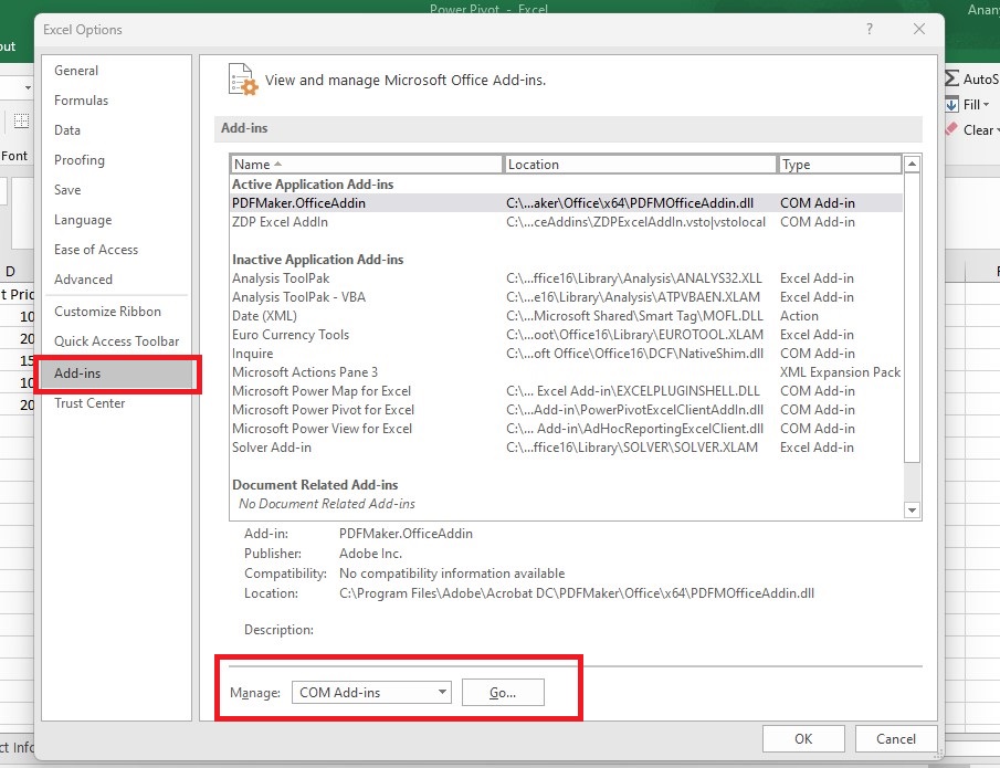
First, go to File > Options > Add-Ins
-
Then, select the Manage box at the bottom, then select COM Add-ins and click Go.
-
You will see 3-4 add-in options. Just check Microsoft Power Pivot for Excel and click OK.
-
A Power Pivot tab will appear on the top ribbon.
Importing Data into Power Pivot
Download this Excel – PowerPivot_Beginner_Example before we proceed further. We will use data from it. This Excel has two tables:
-
Sales Data
Sale ID Product ID Quantity Unit Price 101 1 10 100 102 2 5 200 103 3 8 150 104 1 3 100 105 2 7 200 -
Product Information
Product ID Product Name Category 1 Notebook Stationery 2 Smartphone Electronics 3 Headphones Electronics
From the first table we can tell how many units of each Product ID were sold, but we want to see this data Product Name wise. Meaning – number of units sold for each Product name.
Thus we need to load data into Power Pivot:
-
First select the Sales data table > then go to Power Pivot tab > click Add to Data Model.
-
Repeat this for the Product Info table.
-
Thus the data is loaded and ready to be analyzed using Power Pivot. We can go to Manage in Power Pivot to view the loaded tables.
Creating Relationships and Excel Pivot Table Between Tables
We will now proceed to linking the two tables. We wanted to map the number of units sold against each Product name. One can do it via VLOOKUP or XLOOKUP too. However, Power Pivot does it without writing formulas.
Steps:
-
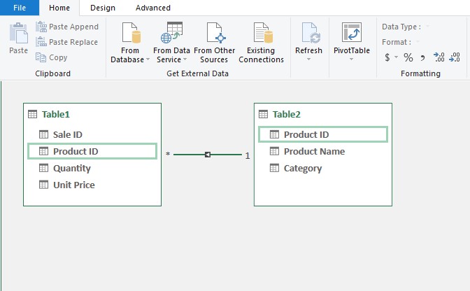
Go to Power Pivot and click Diagram View.
-
Now select the Product ID field from one table and drag and drop it on the Product ID in the other table.
-
You will see that a line is showing showing the relationship.
-
Now return to the Excel sheet and go to Insert > PivotTable.
-
Select Use this workbook’s Data Model.
-
You will notice that you now have the ability to select fields from both the tables into rows, columns, and values fields.
-
Drag Product Name to rows and Quantity to values, just like you would do in a normal pivot table. We will get the desired table telling units sold Product Name wise.
Using DAX to Create Measures
DAX stands for – Data Analysis Expressions. It is a language for writing formulas for Power Pivot. You can think of it as similar to Excel formulas but optimized for data models.
Example: Create a Total Revenue Measure
Have a look at the below formula –
This formula can calculate revenue by multiplying sold quantity column with unit price column, row-by-row. Then it executes the SUMX to give the total sales.
How to Add a Measure:
-
Similar to the procedure we followed for connecting tables, go to the Power Pivot window.
-
Then just select the table where you want to add the measure.
-
Now locate and click on the empty cell in the measure grid and type the above formula.
-
Then press Enter and you will get the total sales.
Benefits of Using Excel Power Pivot
| Feature | Traditional Excel | Power Pivot |
|---|---|---|
| Handles large datasets | Limited | Supports millions of rows |
| Relationships between tables | Manual (VLOOKUP) | Built-in |
| Advanced calculations | Complex formulas | Easy with DAX |
| Performance | Slower | Optimized engine |
Practice Question
Suppose you are a Marketing Analyst who handles ad campaign data from multiple sources, especially –
-
Facebook Ads
-
Google Ads
-
Email campaigns
The problem obviously is that data from each source comes in a different format and has thousands of rows. That is why we can’t manually copy and paste each file in a single sheet as it will become too large. Thus you need to –
-
First import each data source into Power Pivot.
-
Then create relationships between tables using common columns like Campaign ID or Date.
-
Now build a unified Excel PivotTable report with total spend, impressions, and conversions across platforms.
Conclusion
Power Pivot certainly becomes an extremely powerful tool for analysts as the complexity of tasks increases. It can significantly transform the way you work with data.
If you are someone who works with large or multiple data sources, start using Power Pivot today. It’s one of the most powerful tools in Excel’s arsenal.
Also check out our other articles on –
Advanced Filter vs AutoFilter in Excel: What’s the Difference?
Working with Structured Tables in Excel: A Complete Guide
2 thoughts on “Excel Power Pivot for Beginners: Create Data Models Easily”