
VLOOKUP, COUNTIF and SUMIF in Excel are perhaps the most widely used formulas for creating dashboards manually. Pivot tables can create summaries for us without having to write these formulas. However, analysts still use these formulas to create manual summaries for better flexibility.
If you are new to Excel, you may have heard about functions like VLOOKUP, COUNTIF and SUMIF. Excel is a very powerful tool. Despite their somewhat technical sound, these formulas are actually fairly easy to understand once we know how they operate.
I’ll describe each function’s purpose, when to use it, and how to write the formulas using examples from everyday life in this post.
🧐 What Are VLOOKUP, COUNTIF and SUMIF Used For?
-
VLOOKUP – we can search for something in a table and get the corresponding value.
-
COUNTIF – counts how many cells satisfy a given condition in a range.
-
SUMIF – can add up values in a range, but only if they are meeting a specific condition.
Do not worry if you did not understand anything described above. We will discuss in more details, break them down one by one and also provide practical examples.
🔍 1. How to Use VLOOKUP in Excel
What is VLOOKUP?
VLOOKUP stands for “Vertical Lookup.” It is used for searching a cell’s corresponding value from another column in the same table. Let’s see the table in the below – 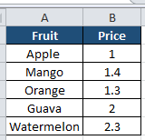
We have fruits and their respective prices. Now if someone asks us the price of Apple we can easily check the table and tell that is is $1. However, when the list of fruits is very long, say 1000 fruits and someone asks us to check the prices of 350 randomly picked fruits from the list, we will not be able to do it manually. Hence we need VLOOKUP.
Syntax:
Basic syntax of VLOOKUP is –
Let’s understand each component with using the same table. We will try to find out the price of Apple with VLOOKUP –
- lookup_value – It is the item whose value we are trying to locate. In our case, it is Apple as we are trying to locate apple’s price.
- table_array – It is the range where apple and its price is located. Hence, we select the entire table having apple. It is important to note we should start the selection from the column having item and the column having value should be on the right side.
- col_index_num – It is the number of column having value. Here it is 2 as the price is the 2nd column from fruit.
- [range_lookup] – Here we can put 0 / false or exact match and 1 / true for approximate match. Meaning, 0 / false will search for apple only and 1 / true will search for apple as well as typos / close matches if any.
Example:
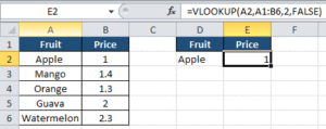
=VLOOKUP(D2, A1:B6, 2, FALSE)
Explanation:
First we enter the lookup_value which is Apple in the second table (D2). This is the cell whose value we are looking for from the 1st table. Then we select the range where the original table is located (A1:B6). Then we enter the column no. of original table where the value is located. In this case, this is the 2nd column of 1st table where price is located. Finally we write FALSE if we want exact match and TRUE for broad match.
Additional Example:
Imagine we have the following data:
| ID | Name | Salary |
|---|---|---|
| 101 | Alex | 50000 |
| 102 | Priya | 55000 |
| 103 | Rohan | 60000 |
Now let’s find out the salary of Priya using her ID.
Formula:
Explanation:
-
102is the value we are looking for (Priya’s ID). -
A2:C4is the table range. -
3means we want the value from the 3rd column (Salary). -
FALSEensures an exact match.
✅ Result: 55000
🔢 2. How to Use COUNTIF in Excel
What is COUNTIF?
COUNTIF helps us in counting how many times a particular item is appearing in a row / column. Or how many items a condition is satisfied in a given range. For example, we can use COUNTIF to count how many times apple is appearing in this list – “apple, orange, apple, guava, apple, watermelon”. Answer is 3.
Syntax:
- range – It is the row / column where we want to count
- criteria – It is the logical test we will run. Here, it is the item we are trying to count (apple).
Example:
Let’s say we have this list of fruits:
| A |
|---|
| Apple |
| Banana |
| Apple |
| Orange |
| Banana |
If we want to count how many times “Banana” appears in this list:
✅ Result: 2
We can also use it with numbers. For example, count how many scores are greater than 70:
| A |
|---|
| 65 |
| 80 |
| 90 |
| 70 |
✅ Result: 2 (Only 80 and 90 are greater than 70)
➕ 3. How to Use SUMIF in Excel
What is SUMIF?
SUMIF can add numbers only if they are meeting a certain condition.
Syntax:
Example:
Here’s a list of products and their sales:
| Product | Sales |
|---|---|
| Pen | 100 |
| Pencil | 150 |
| Pen | 120 |
| Eraser | 80 |
To find out the total sales of Pen, we need to write:
Explanation:
-
A2:A5is the range where we will check the condition. -
"Pen"is the condition. -
B2:B5is the range we want to sum.
✅ Result: 220 (100 + 120)
➕ 4. Bonus Section 1 – SUMIFs in Excel
A more sophisticated variant of SUMIF is called SUMIFS. SUMIFS allows you to add values based on multiple conditions, whereas SUMIF can only add values based on one.This is super useful when you’re working with filtered totals, like:
- Total sales by region and product
- Total points for a particular subject and above a particular threshold
🔧 Syntax:
-
sum_range: This is the row / column we want to add up -
criteria_range1: The range where we will check our first condition -
criteria1: The first condition -
We can add more conditions using more pairs of
criteria_rangeandcriteria
✅ Example 1: Total Sales of “Pen” in “North” Region
Here’s our data for running SUMIF:
| Product | Region | Sales |
|---|---|---|
| Pen | North | 100 |
| Pen | South | 120 |
| Pencil | North | 150 |
| Pen | North | 130 |
| Eraser | North | 80 |
Now we need to calculate the total sales of “Pen” in the “North” region.
Explanation:
-
C2:C6is the range of values we want to sum (Sales) -
A2:A6contains products → we’re checking for “Pen” -
B2:B6contains regions → we’re checking for “North”
✅ Result: 230 (100 + 130)
➕ 5. Bonus Section 2 – COUNTIFs in Excel
COUNTIFS is a more powerful version of COUNTIF. It lets us count cells in a row / column that meet multiple conditions across one or more columns.
We can think of it as: “Count the number of rows where all these conditions are true.”
🔧 Syntax:
-
criteria_range1: The first range to check -
criteria1: The condition for the first range -
We can add more pairs of
criteria_rangeandcriteriaas needed
✅ Example 1: Count Orders for “Pen” in the “North” Region
Here’s our data:
| Product | Region | Quantity |
|---|---|---|
| Pen | North | 10 |
| Pen | South | 12 |
| Pencil | North | 15 |
| Pen | North | 8 |
| Eraser | North | 5 |
We need to count how many times Pen was sold in the North region.
Explanation:
-
A2:A6contains the product names → we are checking for “Pen” -
B2:B6contains regions → we are checking for “North”
✅ Result: 2
(“Pen” + “North” appears in 2 rows)
🎯 Final Thoughts
Some of Excel’s most helpful formulas are VLOOKUP, COUNTIF and SUMIF, particularly if we are just starting out. These allow us to quickly compute totals, count data according to conditions, and search for values.
Try using your own data to practice them; you’ll become more at ease the more you use them!
Please feel free to bookmark this page for future use or share it if you found it useful. Have a query concerning VLOOKUP COUNTIF and SUMIF? Leave a comment with it!
Also read up on more useful formulas like HLOOKUP, XLOOKUP etc here –
Also check out our other articles –
Good.
Good
Awesome
Very good.