
Pivot Tables for beginners can sometimes be a confusing topic. Well, you are not alone if you have ever looked at a disorganized spreadsheet and wondered, “How can I make sense of this and prepare a summary table?”
It is definitely overwhelming to work with a lot of data. Fortunately, pivot tables offer a simple fix.
One of Excel’s (and Google Sheets’) most useful features is the pivot table. Without creating intricate formulas, they assist you in deciphering, summarizing, and analyzing complex data.
Even if this is your first time using Excel, I will cover all you need to know about pivot tables in this tutorial.
Let’s begin!
Table of Contents
-
What is a Pivot Table?
-
Why Should You Use a Pivot Table?
-
How to Prepare Your Data
-
How to Create Your First Pivot Table (Step-by-Step)
-
Understanding the Pivot Table Layout
-
Building Different Pivot Table Reports
-
Common Pivot Table Mistakes Beginners Make
-
Pivot Table Best Practices
-
FAQs About Pivot Tables
-
Practice Exercises
-
Final Thoughts
What is Pivot Tables?
A pivot table is an interactive table that makes it simple for us to arrange, summarize, and evaluate big data sets.
We can answer crucial questions like below ones and organize our data in meaningful ways rather than aimlessly scrolling through thousands of rows:
Q1: In each region, how many products were sold?
Q2: Which salesman generated the most revenue?
Q3: What are the year’s total monthly sales?
All of this is made possible via pivot tables, which eliminate the need for formula writing.
📖 To put it simply, a pivot table spins or “pivots” your data so you may view it from various perspectives.
Why Should You Use Pivot Tables?
Let’s this these real-world scenarios why pivot tables are extremely useful:
| Scenario | Without Pivot Table | With Pivot Table |
|---|---|---|
| We want to find out total sales by each salesperson | We will have to manually add each person’s sales | Just drag one item into a pivot table and it will be calculated in seconds |
| We need to look at monthly trends | We will need to build multiple formulas | Pivot table can automatically group data by month |
| We want to find out errors and patterns | Scroll each row and column manually to spot errors | Prepare summary and quickly spot patterns and outlier values |
To recap: Pivot tables can save lot of time for us. They help in reducing errors, and allow us to focus on insights rather than calculations.
How to Prepare Your Data for Pivot Tables
It is extremely important to set up our data in a correct manner before we start making the pivot table.
Let’s look at a few basic guidelines –
1. Organize data in tabular form for Pivot Tables
Every column should represent a field (For e.g. Name, Date, Sales Amount).
2. Give each column a clear header
Headers are crucial. They are necessary for Excel to comprehend your data.
3. Avoid blank rows and columns
When creating a pivot table in Excel, empty spaces can cause confusion. If we don’t remove empty spaces before creating the pivot tables, we will get empty spaces in summary tables too.
4. Keep data consistent
If we have a “Date” column, we must ensure that every entry is in proper date format – not random text. We can use =DATE(year,month,day) formula for this.
How to Create Your First Pivot Table (Step-by-Step)
Let’s go to the fun part now -we will build our very first pivot table!
Follow along with us these steps carefully:
Step 1: Select Your Data
Click on any cell within your dataset.
🎯 Tip: We do not need to select the entire table manually. We can just click inside anywhere our data table and that will tell Excel that we are ready to create a pivot table.
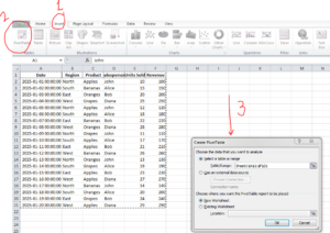
Step 2: Insert Pivot Table
Now go to the top menu bar, then click Insert and then click on PivotTable.
We will see that a new window pops up:
-
Table/Range: Excel will automatically select our data.
-
Choose where to place the pivot table:
-
New Worksheet (This will create a new tab for placing the Pivot table. This is recommended for beginners)
-
Existing Worksheet (Use this if you want it alongside your data)
-
Then Click OK.
Step 3: Understand the Pivot Tables Field List
We will see two things:
-
A blank pivot table will be created. it may look boring for now 🙂
-
A Field List panel will be there on the right side
There are 4 areas in the Field List:
-
Filters: Apply filters across the whole pivot table.
-
Columns: This creates the columns we want in out pivot table. It is the data displayed across the top.
-
Rows: Similarly, this creates the columns we want in out pivot table. This is the data listed down the side.
-
Values: This is the data we want to measure (sum, count, average, etc.).
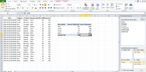
Building Our First Pivot Table
Now let’s say we have this simple data:
| Salesperson | Product | Month | Sales Amount |
|---|---|---|---|
| John | Shoes | Jan | 500 |
| Sarah | Shirts | Jan | 300 |
| Mike | Shoes | Feb | 400 |
Now we can build our pivot table in this manner:
-
Start by dragging Salesperson into Rows.
-
Then drag Sales Amount into Values.
-
(Optional) Drag Month into Columns.
And that is it. Congratulations – we just built our first pivot table! 🎉
It will appear like this:
| Salesperson | Jan | Feb | Grand Total |
|---|---|---|---|
| John | 500 | 500 | |
| Sarah | 300 | 300 | |
| Mike | 400 | 400 |
Exploring Pivot Tables Features
Pivot tables are quite flexible. We can easily do the following with them:
1. Summarize Data in Different Ways
Numbers are summed by default in pivot tables. But we can also:
-
Count (How many times something is appearing in table)
-
Average (Find the mean)
-
Max/Min (Find out highest or lowest value)
We just need to click the drop-down next to “Sum of Sales Amount” and then click Summarize Values By.
2. Sort and Filter
We can also:
-
Apply sort on sales from highest to lowest and vice versa.
-
Apply filter to show only specific salespeople or months.
3. Group Dates
If we have dates (like 01/01/2025, 01/02/2025), we can right-click on the dates and group them:
-
By months
-
By quarters
-
By years
For monthly or quarterly reports, this is a perfect use case.
Common Pivot Tables Mistakes Beginners Make
We have listed some common mistakes people usually make. We should watch out for:
❌ Forgetting to refresh Pivot Tables
If there is some change in our original data, pivot tables will not update automatically. We need to right-click anywhere inside the pivot table and then click Refresh every time.
❌ Using bad data in Pivot Tables
Our pivot table will prepare erroneous results if our data is not clean (For e.g. missing headers, blank rows).
❌ Dragging the wrong fields into Pivot Tables
Beginners can inadvertently enter text values in the Values field.
If “Count of Product” appears in place of “Sum of Sales,” you most likely entered text into Values.
Pivot Tables Best Practices
To become proficient with pivot tables more quickly, use these tips:
- Clean, well-structured data should always come first before creating pivot tables.
- Name your pivot table fields clearly.
- To highlight particular data points, apply filters.
- Employ slicers; doing so makes filtering much simpler.
- To see the data in your pivot table, try using pivot charts.
FAQs About Pivot Tables
Q. Can I update my pivot table if there are changes in my data?
A. Yes, but every time there is a change in date, you must click Refresh manually.
Q. Can I make multiple pivot tables from the same data?
A. Yes we can! Pivot tables, even if originating from same data, are independent of each other once created.
Q. Are pivot tables only available in Excel?
A. No. We can also create them in Google Sheets and other spreadsheet programs.
Q. How do I remove a pivot table?
A. Select the entire pivot table and then press Delete.
Practice Exercises for Pivot Tables
For more practice, here is a sample Excel file you can use to practice more Pivot Tables:
It has columns like Date, Region, Product, Salesperson, Units Sold, and Revenue. It is perfect for creating different types of pivot tables (sums, averages, filters, etc.). Now let’s practice these questions on this Excel –
-
Total Revenue by Region
-
Insert Pivot Table, then drag Region to Rows and Revenue to Values.
-
Find out which Region earned the most.
-
-
Total Units Sold by Product
-
Insert Pivot Table, then drag Product to Rows and Units Sold to Values.
-
Find out the best-selling product.
-
-
Revenue by Salesperson
-
Insert Pivot Table, then drag Salesperson to Rows and Revenue to Values.
-
See who sold the most.
-
Final Thoughts on Pivot Tables
At first, learning pivot tables may seem difficult, but once we get the hang of it, they’re revolutionary. In a matter of minutes, we will be able to evaluate vast amounts of data.
A brief checklist for your pivot table adventure is provided here:
- Start with data that is clean.
- Without worry, drag and drop fields.
- Group, filter, and summarize data.
- Practice various situations.
Whether you deal with data in operations, finance, marketing, or sales, knowing how to use these tables is not simply a “nice-to-have” talent. Rather, it is a must know skill.
Start practicing now by using Google Sheets or Excel.
You’ll be pleasantly shocked at how much simpler your job gets!
Also read up on Pivot Charts – Pivot Charts in Excel
Lean more on Excel and SQL here –
Awesome.
Good.
Good.
Awesome.
Awesome.
Awesome.