
Conditional formatting in Excel is a very helpful tool / technique to make our data visually appealing. We all have been in situations where we are dealing with a confusing Excel sheet that is filled with numbers. Then we wish something would simply stand out to tell us what’s important in that Excel? Conditional formatting does just that – it draws attention to trends, patterns, or trouble spots without requiring us to look through every cell.
This Excel feature can help us save time and make our data much easier to understand, whether we are a student, small business owner, or office warrior.
💡 What is Conditional Formatting?
Conditional Formatting in Excel feature allows us to automatically apply formatting to cells, such as data bars, colors, or icons based on the values within those cells. It’s similar to assigning a visual dress code to your data.
Excel does that for you rather than you having to say, “If this number is greater than 100, I’ll manually highlight it in red.” I mean we can do this manually for 5-10 cells but what if we have 1000s of rows and columns to highlight?
🎯 Why Should You Use It?
-
Spot trends quickly – we can analyze sales data and find out if numbers are growing or dropping
-
Catch errors or outliers – we can spot outliers – unusually high or low values
-
Simplify our analysis – we can draw attention to particular areas using vibrant / pastel colors to show what needs attention
-
Make your reports look professional – As we know, colors and icons = instant readability
🛠️ How to Apply Conditional Formatting
Have a look at below data –
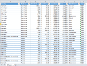
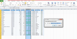
Now let’s say we need to highlight in yellow all gross sales values in E column above $10,000/-. We will –
-
First select our data range (e.g., A1:H50)
-
Then go to the Home tab
-
Now click on Conditional Formatting

-
Choose Highlight Cell Rules > Greater Than
-
Then, just type
$10,000and pick a color -
Click OK – done!
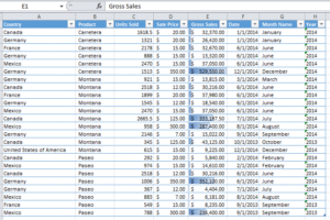
Now, all the cells with values greater than $10,000 will be highlighted.
🔍 Common Types of Conditional Formatting (With Examples)
1. ✅ Highlight Cell Rules
This is same as the above example. We use these to highlight cells based on simple conditions.We can highlight based on greater than, less than, between, equal to, text that contains, duplicate values etc.
Example 2: Highlight Attendance Below 75%
Suppose we have student name in column A and we are tracking student attendance in column B. However, we want to highlight students below 75% attendance.
-
Select column B
-
Then go to Conditional Formatting > Highlight Cell Rules > Less Than
-
Then enter
75%and choose red fill
📌 Useful for teachers, HR teams, or event coordinators!
2. 📈 Top/Bottom Rules
These rules help us in highlighting top performers or under performers with ease.
Example 3: Highlight Top 10 gross sales values
-
Select the gross sales column E
-
Now choose Conditional Formatting > Top/Bottom Rules > Top 10 Items
-
Then write “10” and apply a green fill
🔍 Result: Top 10 gross sales values are now visually marked.
3. 📊 Data Bars
Data bars are surprisingly great for displaying relative performance.
Example 4: Add Data Bars to Revenue Data
-
Select column E containing gross sales
-
Now go to Conditional Formatting > Data Bars
-
Then pick a gradient fill, which is the style and color of our choice
🎯 Tip: This cool feature converts our numbers into mini bar charts which is great for dashboards!
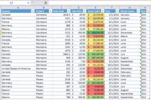
4. 🌈 Color Scales
Color Scales are our personal favorite. They can straightaway create a heatmap-like effect where colors reflect value intensity.
Example 5: Apply Color Scales to gross sales
-
Select E column
-
Then choose Conditional Formatting > Color Scales > Green-Yellow-Red
🔍 Green = High value, Red = Low margin – extremely useful in financial analysis!
5. 🚦 Icon Sets
These add symbols like arrows, traffic lights, or stars to show value categories.
Example 6: Use Icon Sets for units sold
-
First select unites sold meaning C column
-
Then go to Conditional Formatting > Icon Sets > 3 Stars
⭐ Thus, looking at this data become more visual and fun!

📏 Advanced: Use Formula-Based Conditional Formatting
Do you want to highlight rows based on a condition in another column? We can use a formula.
Example 7: Highlight Delayed Projects
Suppose we have a project tracker where:
-
Column A = Project Name
-
Column B = Status (“On Track”, “Delayed”, “Completed”)
Now we want to highlight the entire row where status is Delayed.
Steps:
-
Select the full table
-
Now go to Conditional Formatting > New Rule
-
Then choose Use a formula to determine which cells to format
-
Enter:
=$B2="Delayed" -
Then pick red fill, click OK
✅ Now the rows where delayed project is mentioned will be automatically flagged.
🧽 How to Remove Conditional Formatting
Removing conditional formatting in Excel is easy. Here is how –
-
Select your range
-
Go to Conditional Formatting > Clear Rules
-
Then choose Clear Rules from Selected Cells
⚠️ Pro Tips for Better Formatting
- Employ subdued hues: Unless you’re writing a report with a disco theme, stay away from neon!
- Conditional formatting in Excel is a heavy feature. Hence, to prevent damaging large sheets, test formulas on a small set first.
- For deeper insights, combine with pivot tables and filters.
- To lock columns or rows as needed, use cell references in formulas (such as $B2).
🚀 Final Thoughts
Conditional formatting in Excel helps us work more efficiently, not just make our Excel sheet look nice. These formatting guidelines help us quickly focus on what really matters, whether you’re managing sales, keeping tabs on spending, or planning projects.
You’ll soon be making dashboards that not only function but also look amazing if you start with the fundamentals and experiment with the rules.
✅ [Practice Excel Sheet Description]
Sheet Name: Sales Data
| Region | Sales Rep | Product | Units Sold | Unit Price | Total Sales | Target |
|---|---|---|---|---|---|---|
| North | Alice | Laptop | 30 | 55000 | 1650000 | 1500000 |
| South | Bob | Phone | 100 | 25000 | 2500000 | 2000000 |
| East | Charlie | Tablet | 50 | 30000 | 1500000 | 1800000 |
| West | David | Monitor | 40 | 15000 | 600000 | 750000 |
| North | Emily | Laptop | 25 | 55000 | 1375000 | 1400000 |
We can practice below mentioned questions on conditional formatting in Excel from this table –
📝 List of Practice Questions for Conditional Formatting
Beginner Level:
-
Highlight all rows in green where
Total Salesis greater thanTarget. -
Highlight in red all those cells where
Total Salesis less thanTarget. -
Make use of color scales to represent
Units Sold(green for high, red for low). -
Highlight duplicates in the
Regioncolumn. -
Apply a yellow fill to the
Productcolumn where the product is “Laptop”.
Intermediate Level:
- Use an icon set to display performance: ✅ if Total Sales >= Target, ❌ otherwise.
- Create a rule that highlights rows where the
Sales Repname starts with the letter “D”. - Use a custom formula to highlight rows where
Total Salesis 10% less thanTarget. Formula:=F2<(G2*0.9) - Apply conditional formatting to the entire row if the
Regionis “East”. - Use a data bar to visualize
Unit Price.
Advanced Level:
- Highlight the top 2
Total Salesfigures in blue. - Create a heat map of the
Units Soldcolumn using color scales. - Highlight rows where the
Productis “Laptop” andTotal Salesis below target. - Use a formula to highlight reps whose sales are within 5% of the target. – Formula:
=ABS(F2-G2)<=G2*0.05 - Use conditional formatting to flag any blank cells in the table.
Drop your queries in the comment box and we will promptly answer those. Also read up more on conditional formatting here –
Conditional Formatting Official Guide
Also check out our other articles on –
Awesome.
Good.
Good.
Good.
Good.
Awesome.
Awesome.
Very good.